This is the real method that actually constructs the graph. While we will not go through every single line in details we will highlight the complications and some formatting options we have used.
In order to create the colored background we create filled area plots and add them to the graph. Starting with the "brown" and successively adding the rest to create the colored band effect we want. Figure 31.6 shows in "slow-motion" how this is done by adding four area plots, one at a time.
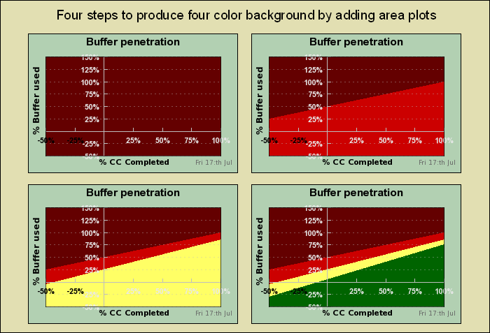
The exact position for the lines are calculated with the positions given for each color band. The position for each color band is specified by giving the y-coordinate at x=0 and the y-coordinate at the maximum x-scale value.
When adding the area plots there is one thing we have to modify. By default the fill is done between the line and the y=0 line. In our case we need the fill to go all the way down to the min y-value. To change this behavior we need to call the method
LinePlot::SetFillFromYMin()
for each of the areas.
Since we want some discrete horizontal grid lines we might think that it is enough to do the normal
1 | $graph->ygrid->Show(); |
However, doing that will not show any grid lines. The reason is hat by default the grid lines are drawn at the bottom of the plot. Since we have filled area plots covering 100% of the pot area no grid lines would show. In order to change this we need to move the grid line to the front with a call to the method
Graph::SetGridDepth($aDepth)
using the argument DEPTH_FRONT. The rest of the grid line
formatting is just basic style and color modification to make the grid visible
but just barely.
For this type of graph we have manually set the distance between each tick label to 25 units. This would put labels as 0,25,50, and so on. The maximum value (the user specifies) will be adjusted so that it is always an even multiple of 25 to allow the last tick mark to be at the end of the axis.
As can be seen from the previous images we are using one feature that hasn't been previously exemplified and that is the possibility to have unique colors on each label on the scale. We use this for the x-scale by having the negative labels in black and the positive labels in white. The reason is purely functional to allow the scale labels to be more easy to read against the colored background.
The color of the labels are specified as the second argument to
Axis::SetColor($aAxisColor,$aLabelColor)
In addition we have also hidden the zero labels since they would just be disturbing in the middle and doesn't really add any information we don't already have.
Finally the labels are formatted to show a percentage sign after each label. This is done by a format string
In the beginning of the Init() method the margins for the graph
is adjusted depending on the actual size the user specified. The same goes with
establishing the basic font size used for the scale labels as well as the titles
(both graph and axis). The size is just based on heuristics on what (in our
view) gives a well balanced graph.